HistogramZoo

Introduction

The HistogramZoo R package is a collection of functions which aim to identify and characterize patterns from histogram data.

The Histogram and GenomicHistogram class

A Histogram object contains 1 piece of essential data and 4 pieces of optional data:

histogram_data is a numeric vector representing histogram data. In cases of equal bin width, histogram_data can equally represent counts or density with no functional differences. However, in cases of unequal bin width, only density is appropriate for distribution fitting and visualization.
interval_start and histogram_end are numeric vectors representing the start and end coordinates of each bin
bin_width is the numeric length of bins. This can be automatically estimated from interval_start and interval_end. Objects are required to have equal bin width for every bin with the exception of the last bin, which can have a shorter bin width.
region_id is a character id for the histogram

A GenomicHistogram object contains up to 6 additional pieces of data.

chr is a character chromosome
strand is a character strand which is restricted to one of +, - and *
intron_start and intron_end are numeric vectors representing intron coordinates - these can be automatically computed based on non-consecutive interval_start and interval_end indices
consecutive_start and consecutive_end are numeric vectors representing a continuous intronless bin coordinate system on which summary statistics can be computed and distributions can be fitted. Optionally specified by the user, consecutive_start/end will be automatically generated based on provided interval_start/end and intron data starting at base 1.

A Histogram and a GenomicHistogram differ in several ways:

Conceptualization of bins: Histogram objects represent conventional histograms where data are binned on a real number scale. Bins are of the form (start, end] where starts are inclusive while ends are exclusive with the exception of the last bin where both start and end are inclusive. GenomicHistogram objects were designed to represent a discrete base 1 system where each histogram bin represents a set of indices on which observations are collected.
Only GenomicHistogram objects support the use of disjoint intervals, or non-consecutive bins. This feature was designed with GenomicHistogram objects in mind to support the representation of transcripts and genes as a set of exons which might not be consecutive intervals on the genomic coordinate system. Summary statistics and distributions are fit on consecutive_start/end coordinates for GenomicHistograms. In operational cases using consecutive bins, consecutive_start/end can be specified to be the same as interval_start/end.

my_histogram <- Histogram(
  histogram_data = c(1,2,3,1,5,6),
  interval_start = c(0,1,2,3,4,5),
  interval_end = c(1,2,3,4,5,6),
  bin_width = 1,
  region_id = "my_histogram"
)

create_coverageplot(
  my_histogram,
  main.cex = 1,
  xaxis.tck = 0, 
  yaxis.tck = 0, 
  xlab.cex = 1, 
  ylab.cex = 1, 
  xaxis.cex = 0.8, 
  yaxis.cex = 0.8,
  xat = generate_xlabels(my_histogram, n_labels = length(my_histogram), return_xat = T), 
  xaxis.lab = generate_xlabels(my_histogram, n_labels = length(my_histogram)), 
)

my_genomic_histogram <- GenomicHistogram(
  histogram_data = c(4,5,2,3,6,8),
  interval_start = c(1:3, 5:7),
  interval_end = c(1:3, 5:7),
  bin_width = 1,
  region_id = "my_genomic_histogram",
  chr = "chr1",
  strand = "*",
  intron_start = c(4),
  intron_end = c(4),
  consecutive_start = seq(6),
  consecutive_end = seq(6)
)

create_coverageplot(
  my_genomic_histogram,
  main.cex = 1,
  xaxis.tck = 0, 
  yaxis.tck = 0, 
  xlab.cex = 1, 
  ylab.cex = 1, 
  xaxis.cex = 0.8, 
  yaxis.cex = 0.8,
  xat = generate_xlabels(my_genomic_histogram, n_labels = length(my_genomic_histogram), return_xat = T), 
  xaxis.lab = generate_xlabels(my_genomic_histogram, n_labels = length(my_genomic_histogram)), 
)

Estimation of summary statistics

Built-in functions can be used to estimate summary statistics, including a weighted mean, variance, standard deviation and skew, on each Histogram object.

histogram_summary <- data.frame(
  "id" = "my_histogram",
  "mean" = weighted.mean(my_histogram),
  "var" = weighted.var(my_histogram),
  "sd" = weighted.sd(my_histogram),
  "skew" = weighted.skewness(my_histogram)
)

genomic_histogram_summary <- data.frame(
  "id" = "my_genomic_histogram",
  "mean" = weighted.mean(my_genomic_histogram),
  "var" = weighted.var(my_genomic_histogram),
  "sd" = weighted.sd(my_genomic_histogram),
  "skew" = weighted.skewness(my_genomic_histogram)

)

knitr::kable(
  rbind(histogram_summary, genomic_histogram_summary)
)

id	mean	var	sd	skew
my_histogram	3.888889	2.722222	1.649916	-0.5943331
my_genomic_histogram	3.928571	3.550265	1.884215	-0.3173915

Data loaders

Data loaders for `Histogram` objects

observations_to_histogram bins a set of observations at a designated histogram_bin_width to generate a Histogram

set.seed(314)
my_data <- rnorm(10000, mean = 10, sd = 5)
my_histogram <- observations_to_histogram(my_data, histogram_bin_width = 1)

create_coverageplot(
  my_histogram, 
  main.cex = NULL, 
  xaxis.tck = 0, 
  yaxis.tck = 0, 
  xlab.cex = 1, 
  ylab.cex = 1, 
  xaxis.cex = 0.8, 
  yaxis.cex = 0.8
)

Data loaders for `GenomicHistogram` objects

bigWig_to_histogram bins the coverage from a single bigWig file on a set of user-defined regions (provided as a GRanges object, a GRangesList* object or a GTF file) and returns a list of GenomicHistogram objects.

library(GenomicRanges)

filename <- system.file("extdata", "bigwigs",  "S1.bw", package = "HistogramZoo")

regions <- GenomicRanges::GRanges(
  seqnames = "chr1",
  IRanges::IRanges(
    start = c(17950, 19350),
    end = c(18000, 19600)),
  strand = "*"
)

bigwig_histograms <- bigWig_to_histogram(
  filename = filename,
  regions = regions,
  histogram_bin_size = 10
)

genome_BED_to_histogram bins the coverage from a set of genomic BED files and returns a list of GenomicHistogram objects. Users have the option of providing a set of regions as a GRanges or GRangesList* object.

datadir <- system.file("extdata", "dna_bedfiles",  package = "HistogramZoo")
genome_bed_files <- list.files(datadir, pattern = ".bed$")
genome_bed_files <- file.path(datadir, genome_bed_files)

genome_bed_histograms <- genome_BED_to_histogram(
  filenames = genome_bed_files,
  n_fields = 6,
  histogram_bin_size = 1
)

transcript_BED_to_histogram, to account for overlapping transcript annotations, bins the coverage on a set of BED files where each element can be pre-assigned to a region using the 4th column (name) of the BED file.

datadir <- system.file("extdata", "rna_bedfiles", package = "HistogramZoo")
transcript_bed_files <- file.path(datadir, paste0("Sample.", 1:20, ".bed"))
gtf <- system.file("extdata", "genes.gtf", package = "HistogramZoo")

histograms <- transcript_BED_to_histogram(
  filenames = transcript_bed_files,
  n_fields = 12,
  gtf = gtf,
  gene_or_transcript = "gene",
  histogram_bin_size = 10
)

Notes on common parameters

regions [bigWig, genomic BED]: Using a GRangesList object allows the assignment of disjoint intervals to a GenomicHistogram (e.g. representing a set of exons that can be joined to form a mature transcript) where each GRanges object in the GRangesList represents the elements of a single Histogram. Using a GRanges object creates a separate GenomicHistogram for each element in the GRanges object.
histogram_bin_size [bigWig, genomic and transcriptomic BED]: Bins are generated using GenomicRanges::tile and coverage is calculated using GenomicRanges::binnedAverage. This strategy strives to create bins of equal size less than or equal to the designated histogram_bin_size (see above for discussion of the difference in bin_width restriction.)
allow_overlapping_segments_per_sample [transcriptomic and genomic BED]: Each BED file is assumed to contain the elements of a single experimental sample. Thus, overlapping elements in each BED file can be eliminated by setting the parameter to FALSE.

Segmentation and distribution fitting

The function segment_and_fit is designed to be a pipeline constructed from the following sub-functions which enables the segmentation, denoising and fitting of statistical distributions on Histogram and GenomicHistogram objects. Each of the parameters in segment_and_fit have counterparts in the sub-functions which is explored in further detail below.

NOTA BENE: Most of the functions below are implemented as S3 methods which can take Histogram, GenomicHistogram and numeric vector objects as input.

Finding local optima

find_local_optima identifies the local minima and maxima on a vector of counts (histogram data).

# Generating a Histogram 
set.seed(314)
dt = rnorm(10000, mean = 20, sd = 10)
xhist = observations_to_histogram(dt, histogram_bin_width = 2)

# basic use
optima = find_local_optima(xhist)
optima = sort(unlist(optima))

create_coverageplot(
  xhist, 
  add.points = T, 
  points.x = optima, 
  points.y = xhist$histogram_data[optima], 
  points.col = "red",
  main = "basic optima",
  main.cex = 1, 
  xaxis.tck = 0, 
  yaxis.tck = 0, 
  xlab.cex = 1, 
  ylab.cex = 1, 
  xaxis.cex = 0.8, 
  yaxis.cex = 0.8
)

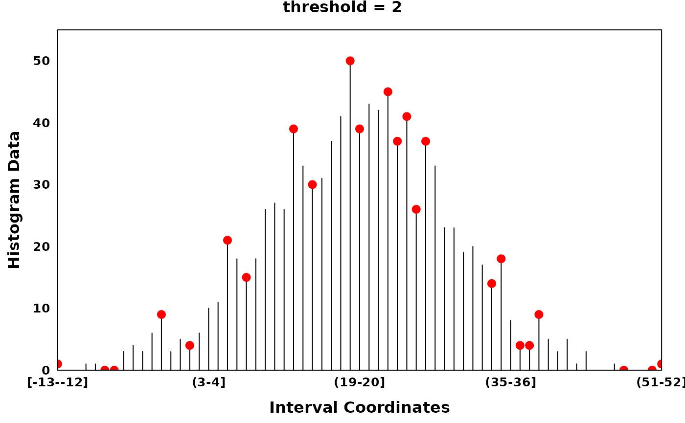
The parameter threshold allows the user to tune the sparsity of local optima to histograms with potentially noisy counts, i.e. by thresholding the difference between neighbouring optima.

# Generating a Histogram with noisy counts
set.seed(314)
dt = rnorm(1000, mean = 20, sd = 10)
xhist = observations_to_histogram(dt, histogram_bin_width = 1)

# find_local_optima with threshold 0
zero_threshold_optima = find_local_optima(xhist, threshold = 0)
zero_threshold_optima = sort(unlist(zero_threshold_optima))

create_coverageplot(
  xhist,
  add.points = T, 
  points.x = zero_threshold_optima,
  points.y = xhist$histogram_data[zero_threshold_optima],
  points.col = "red", 
  type = "h",
  main = "threshold = 0",
  main.cex = 1, 
  xaxis.tck = 0, 
  yaxis.tck = 0, 
  xlab.cex = 1, 
  ylab.cex = 1, 
  xaxis.cex = 0.8, 
  yaxis.cex = 0.8
)

# find_local_optima with threshold 2
threshold_optima = find_local_optima(xhist, threshold = 2)
threshold_optima = sort(unlist(threshold_optima))

create_coverageplot(
  xhist, 
  add.points = T, 
  points.x = threshold_optima, 
  points.y = xhist$histogram_data[threshold_optima], 
  points.col = "red", 
  type = "h",
  main = "threshold = 2",
  main.cex = 1, 
  xaxis.tck = 0, 
  yaxis.tck = 0, 
  xlab.cex = 1, 
  ylab.cex = 1, 
  xaxis.cex = 0.8, 
  yaxis.cex = 0.8
)

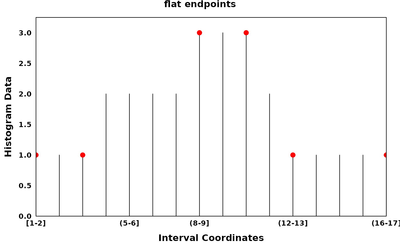
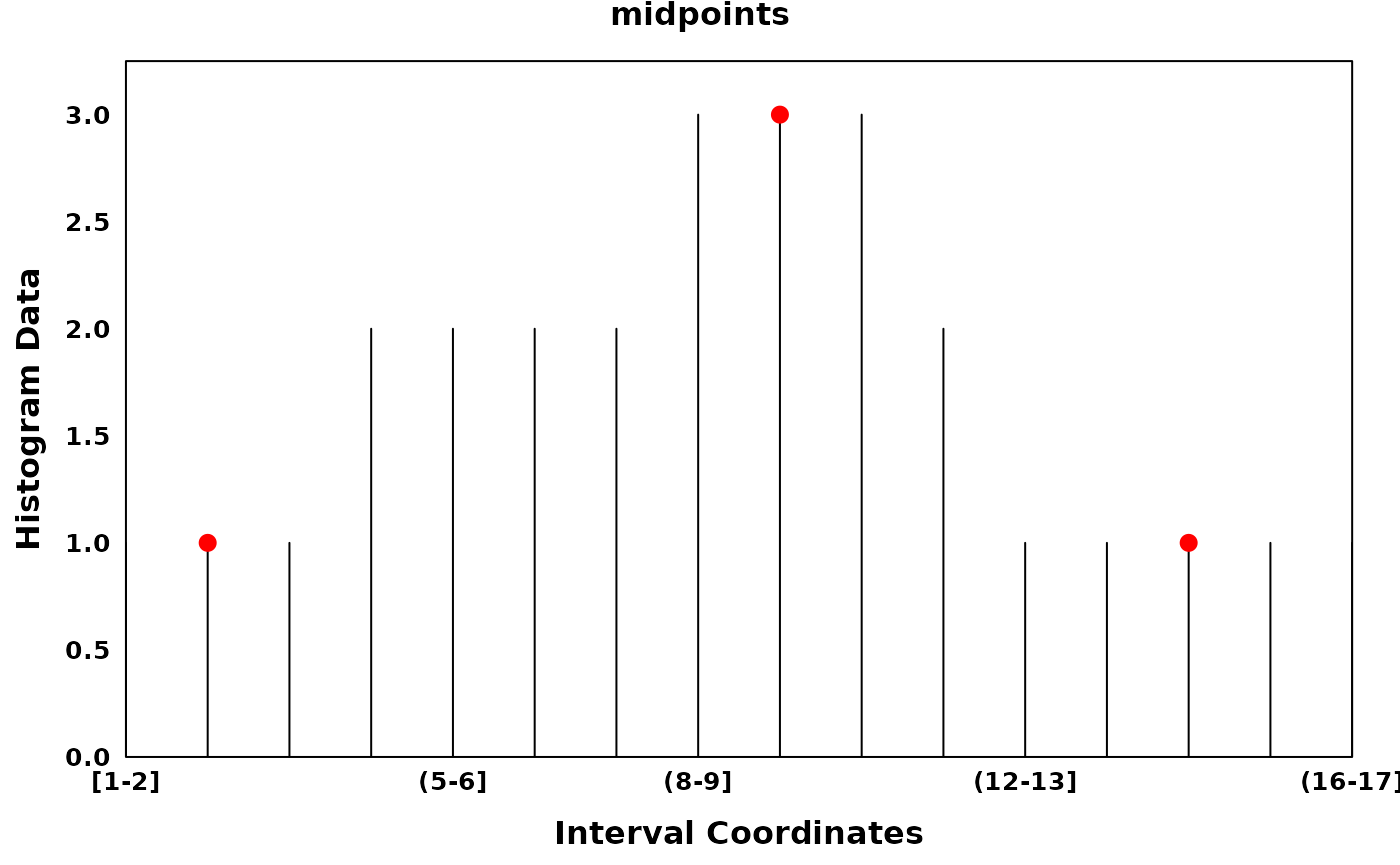
The parameter flat_endpoints allows the user to better fit histograms with stretches of equal values (e.g. pile-ups of BED files in a GenomicHistogram). Setting the parameter to TRUE will allow the user to return both endpoints of a flat region while setting the parameter to FALSE will return the estimated midpoint of a flat region.

# Generating a Histogram with consecutive equal values
data = c(rep(1, 3), rep(2, 4), rep(3, 3), rep(2, 1), rep(1, 5))
xhist = Histogram(histogram_data = data)

# flat_endpoints
optima_flat = find_local_optima(xhist, flat_endpoints = TRUE)
optima_flat = sort(unlist(optima_flat))

create_coverageplot(
  xhist, 
  add.points = T, 
  points.x = optima_flat, 
  points.y = xhist$histogram_data[optima_flat], 
  points.col = "red",
  main = "flat endpoints",
  main.cex = 1, 
  xaxis.tck = 0, 
  yaxis.tck = 0, 
  xlab.cex = 1, 
  ylab.cex = 1, 
  xaxis.cex = 0.8, 
  yaxis.cex = 0.8
)

# midpoints
optima_midpoints = find_local_optima(xhist, flat_endpoints = FALSE)
optima_midpoints = sort(unlist(optima_midpoints))

create_coverageplot(
  xhist, 
  add.points = T, 
  points.x = optima_midpoints, 
  points.y = xhist$histogram_data[optima_midpoints], 
  points.col = "red",
  main = "midpoints",
  main.cex = 1, 
  xaxis.tck = 0, 
  yaxis.tck = 0, 
  xlab.cex = 1, 
  ylab.cex = 1, 
  xaxis.cex = 0.8, 
  yaxis.cex = 0.8
)

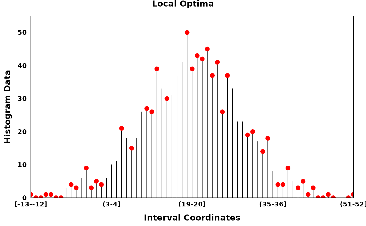
The Fine-to-Coarse segmentation algorithm

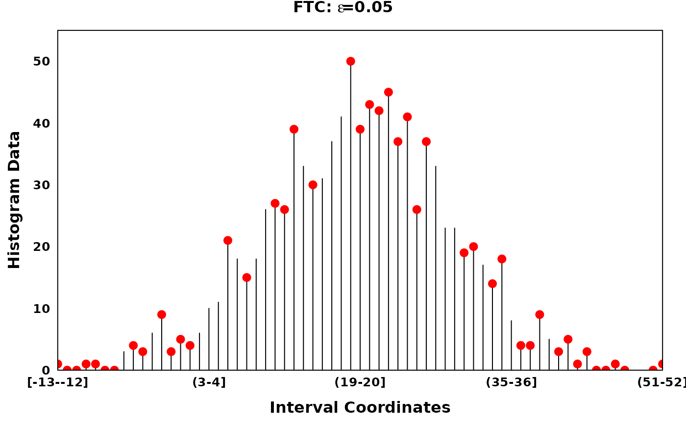
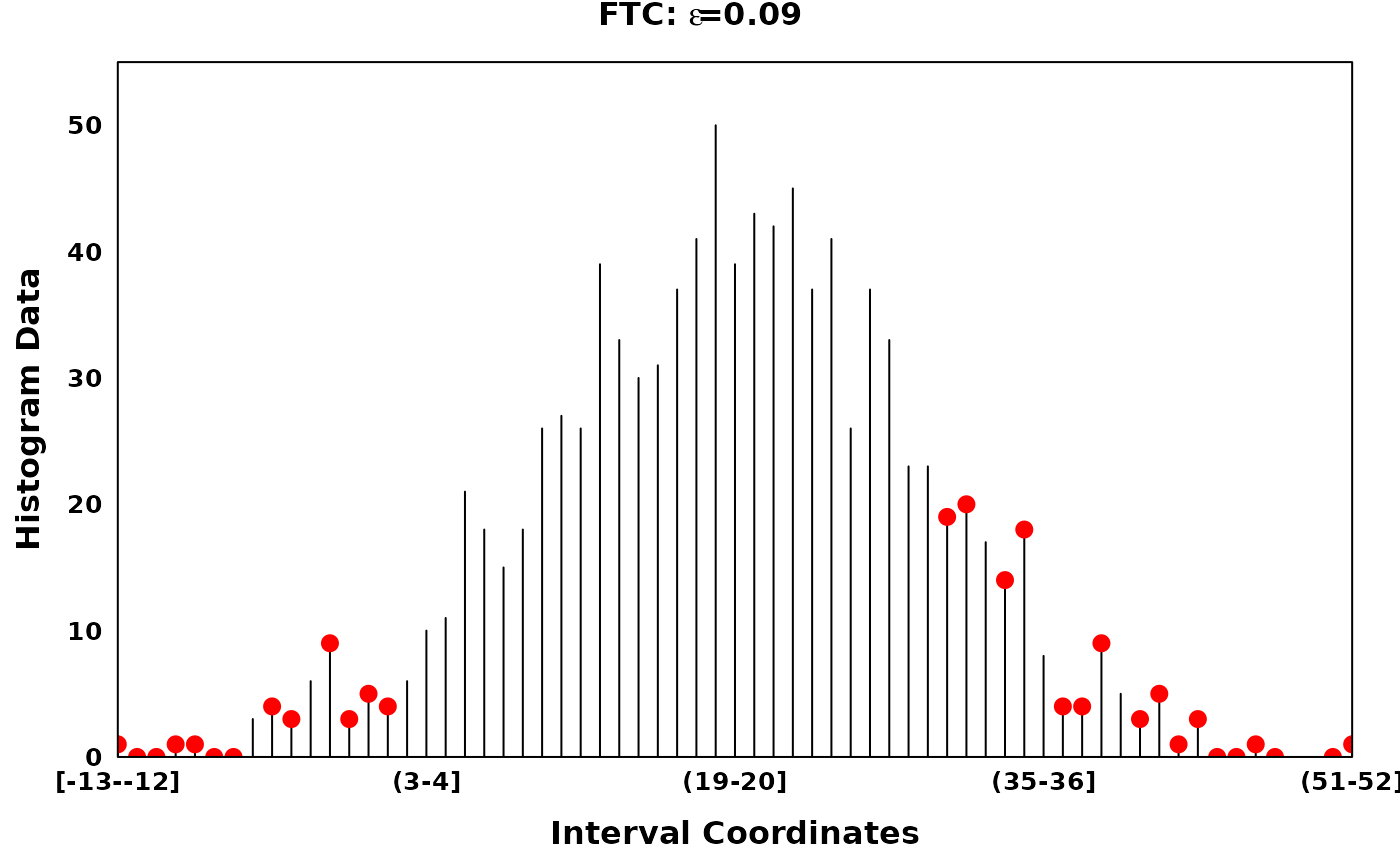
The Fine-to-Coarse segmentation algorithm was described in Delon et al. (2005), Lisani and Petro (2021) and Delon et al. (2006). Briefly, for a given histogram and a set of local optima, the FTC algorithm iterates through consecutive segments identifying peaks, segments of increasing counts followed by segments of decreasing counts. Consecutive segments are merged based on the prioritization derived from a monotone cost function, until an optimal set of peaks are acquired. Granularity of the optimal peak set can be tuned via the hyperparamter \(\epsilon\).

# Generating a Histogram with noisy counts
set.seed(314)
dt = rnorm(1000, mean = 20, sd = 10)
xhist = observations_to_histogram(dt, histogram_bin_width = 1)

# local optima
zero_threshold_optima = find_local_optima(xhist, threshold = 0)
zero_threshold_optima = sort(unlist(zero_threshold_optima))

create_coverageplot(
  xhist,
  add.points = T, 
  points.x = zero_threshold_optima,
  points.y = xhist$histogram_data[zero_threshold_optima],
  points.col = "red", 
  type = "h",
  main = "Local Optima",
  main.cex = 1, 
  xaxis.tck = 0, 
  yaxis.tck = 0, 
  xlab.cex = 1, 
  ylab.cex = 1, 
  xaxis.cex = 0.8, 
  yaxis.cex = 0.8
)

# Using different epsilons on FTC
ftc_eps_0.05 <- ftc(xhist, s = zero_threshold_optima, eps = 0.05)
ftc_eps_0.09 <- ftc(xhist, s = zero_threshold_optima, eps = 0.09)
ftc_eps_0.15 <- ftc(xhist, s = zero_threshold_optima, eps = 0.15)
ftc_eps_0.25 <- ftc(xhist, s = zero_threshold_optima, eps = 0.25)
ftc_eps_0.5 <- ftc(xhist, s = zero_threshold_optima, eps = 0.5)

create_coverageplot(
  xhist,
  add.points = T, 
  points.x = ftc_eps_0.05,
  points.y = xhist$histogram_data[ftc_eps_0.05],
  points.col = "red", 
  type = "h",
  main = expression(bold(paste("FTC: ", epsilon, "=0.05"))),
  main.cex = 1, 
  xaxis.tck = 0, 
  yaxis.tck = 0, 
  xlab.cex = 1, 
  ylab.cex = 1, 
  xaxis.cex = 0.8, 
  yaxis.cex = 0.8
)

create_coverageplot(
  xhist,
  add.points = T, 
  points.x = ftc_eps_0.09,
  points.y = xhist$histogram_data[ftc_eps_0.09],
  points.col = "red", 
  type = "h",
  main = expression(bold(paste("FTC: ", epsilon, "=0.09"))),
  main.cex = 1, 
  xaxis.tck = 0, 
  yaxis.tck = 0, 
  xlab.cex = 1, 
  ylab.cex = 1, 
  xaxis.cex = 0.8, 
  yaxis.cex = 0.8
)

create_coverageplot(
  xhist,
  add.points = T, 
  points.x = ftc_eps_0.15,
  points.y = xhist$histogram_data[ftc_eps_0.15],
  points.col = "red", 
  type = "h",
  main = expression(bold(paste("FTC: ", epsilon, "=0.15"))),
  main.cex = 1, 
  xaxis.tck = 0, 
  yaxis.tck = 0, 
  xlab.cex = 1, 
  ylab.cex = 1, 
  xaxis.cex = 0.8, 
  yaxis.cex = 0.8
)

create_coverageplot(
  xhist,
  add.points = T, 
  points.x = ftc_eps_0.25,
  points.y = xhist$histogram_data[ftc_eps_0.25],
  points.col = "red", 
  type = "h",
  main = expression(bold(paste("FTC: ", epsilon, "=0.25"))),
  main.cex = 1, 
  xaxis.tck = 0, 
  yaxis.tck = 0, 
  xlab.cex = 1, 
  ylab.cex = 1, 
  xaxis.cex = 0.8, 
  yaxis.cex = 0.8
)

create_coverageplot(
  xhist,
  add.points = T, 
  points.x = ftc_eps_0.5,
  points.y = xhist$histogram_data[ftc_eps_0.5],
  points.col = "red", 
  type = "h",
  main = expression(bold(paste("FTC: ", epsilon, "=0.5"))),
  main.cex = 1, 
  xaxis.tck = 0, 
  yaxis.tck = 0, 
  xlab.cex = 1, 
  ylab.cex = 1, 
  xaxis.cex = 0.8, 
  yaxis.cex = 0.8
)

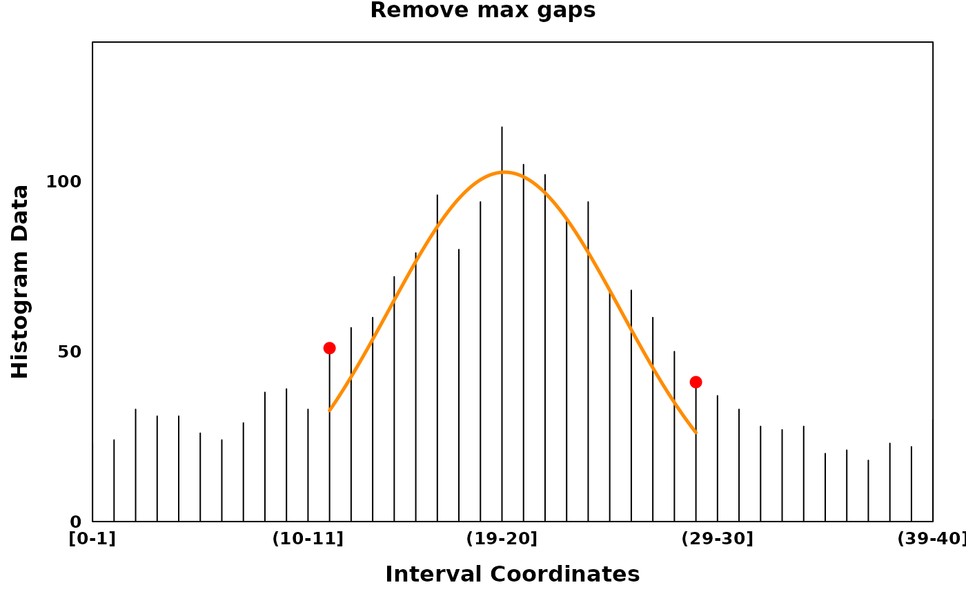
Filtering low entropy regions

In the presence of noisy data, it can be helpful to filter regions with low entropy to extract high density regions. Low entropy regions or max_gaps can be identified using the algorithm described in Delon et al. (2005). Briefly, a region is defined as a gap if it has high entropy and low density relative to its adjacent peak. Identification of max gaps is conducted on each segment post-segmentation.

# Generating a Histogram with noisy counts
set.seed(314)
dt = c(
  rnorm(1000, mean = 20, sd = 5),
  runif(1000, min = 0, max = 40)
)
xhist = observations_to_histogram(dt, histogram_bin_width = 1)

# Segment and Fit with and without filtering for max gaps
filtered_fit <- segment_and_fit(
  histogram_obj = xhist,
  eps = 1,
  seed = 314,
  remove_low_entropy = TRUE,
  metric = c("jaccard", "intersection", "ks", "mse", "chisq")
)

unfiltered_fit <- segment_and_fit(
  histogram_obj = xhist,
  eps = 1,
  seed = 314,
  remove_low_entropy = FALSE,
  metric = c("jaccard", "intersection", "ks", "mse", "chisq")
)

unfiltered_plt <- create_coverageplot(
  unfiltered_fit,
  main = "Unfiltered",
  main.cex = 1, 
  xaxis.tck = 0, 
  yaxis.tck = 0, 
  xlab.cex = 1, 
  ylab.cex = 1, 
  xaxis.cex = 0.8, 
  yaxis.cex = 0.8,
  legend = NULL
)

# Plotting
filtered_plt <- create_coverageplot(
  filtered_fit,
  main = "Remove max gaps",
  main.cex = 1, 
  xaxis.tck = 0, 
  yaxis.tck = 0, 
  xlab.cex = 1, 
  ylab.cex = 1, 
  xaxis.cex = 0.8, 
  yaxis.cex = 0.8,
  legend = NULL
)

print(unfiltered_plt)
print(filtered_plt)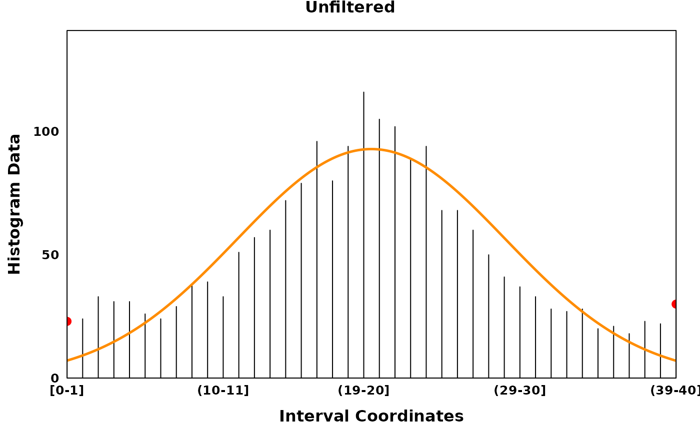

Fitting statistical distributions

Distributions

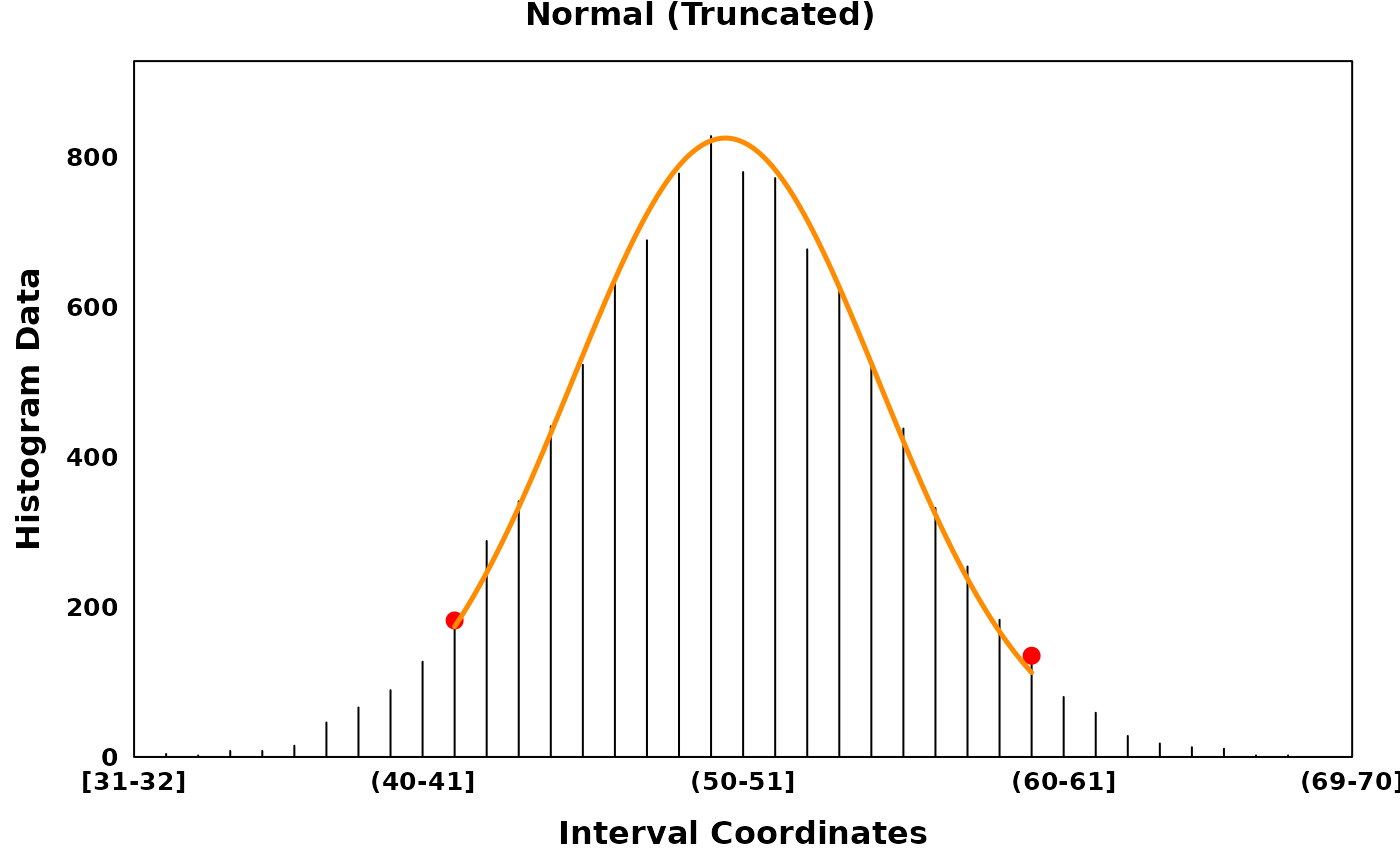
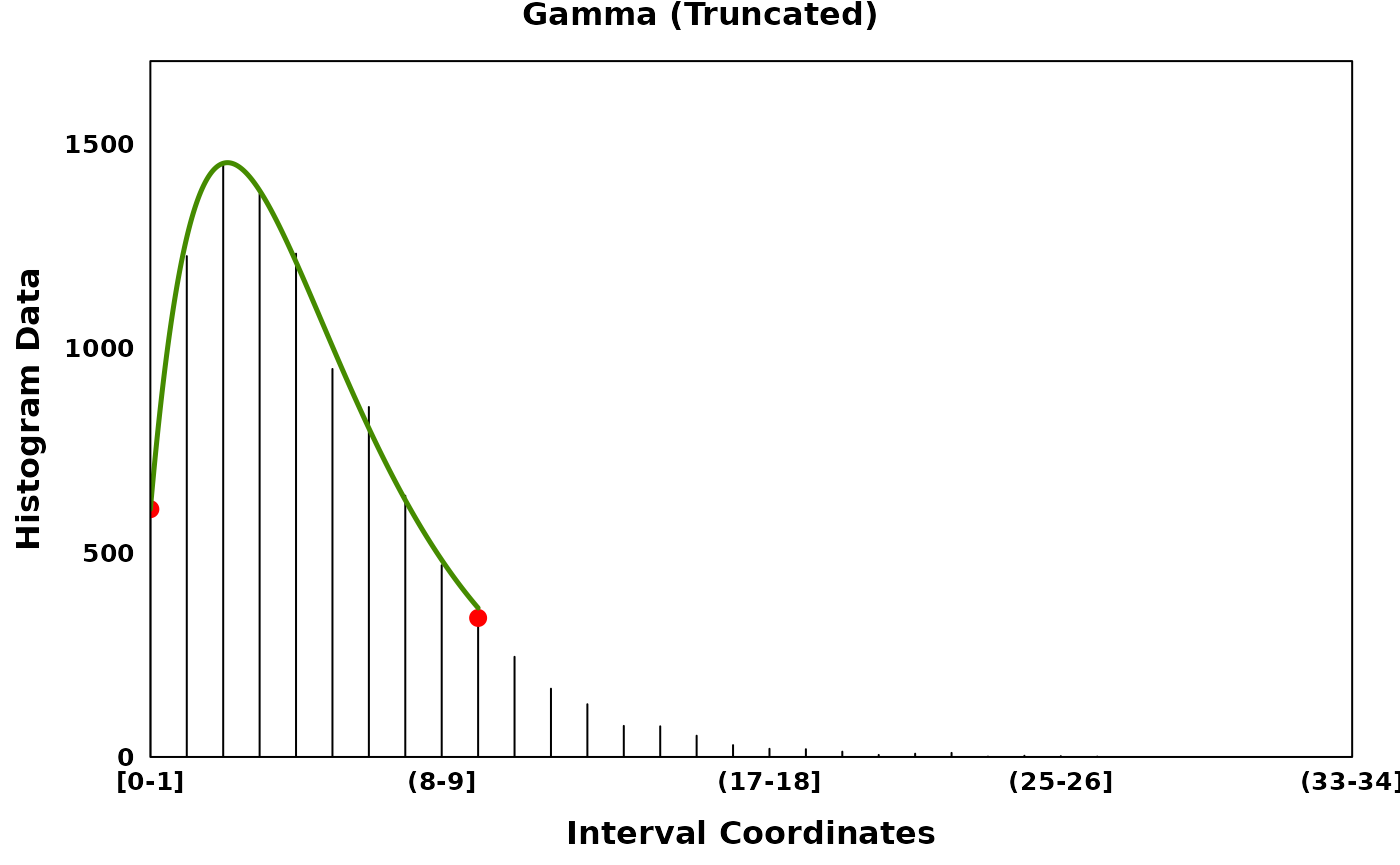
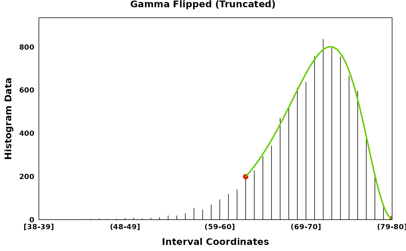
Three distributions are provided: the normal (Gaussian) distribution, the uniform distribution and the gamma distribution. The gamma distribution can be flipped to account for skew in the negative direction. Normal and gamma distributions can be fit in their full form or in a truncated form.

set.seed(314)
gaussian_data <- rnorm(10000, mean = 50, sd = 5)
gaussian_histogram <- observations_to_histogram(gaussian_data)

# Keeping all data and fitting a full model
gaussian_full <- segment_and_fit(
  histogram_obj = gaussian_histogram,
  eps = 1,
  seed = 314,
  remove_low_entropy = FALSE,
  truncated_models = FALSE,
  metric = c("jaccard", "intersection", "ks", "mse", "chisq")
)

# Removing noisy data and fitting a truncated model
gaussian_truncated <- segment_and_fit(
  histogram_obj = gaussian_histogram,
  eps = 1,
  seed = 314,
  remove_low_entropy = TRUE,
  truncated_models = TRUE,
  metric = c("jaccard", "intersection", "ks", "mse", "chisq")
)

gaussian_full_plt <- create_coverageplot(
  gaussian_full,
  main = "Normal (Full)",
  main.cex = 1, 
  xaxis.tck = 0, 
  yaxis.tck = 0, 
  xlab.cex = 1, 
  ylab.cex = 1, 
  xaxis.cex = 0.8, 
  yaxis.cex = 0.8,
  legend = NULL
)

gaussian_truncated_plt <- create_coverageplot(
  gaussian_truncated,
  main = "Normal (Truncated)",
  main.cex = 1, 
  xaxis.tck = 0, 
  yaxis.tck = 0, 
  xlab.cex = 1, 
  ylab.cex = 1, 
  xaxis.cex = 0.8, 
  yaxis.cex = 0.8,
  legend = NULL
)

print(gaussian_full_plt)
print(gaussian_truncated_plt)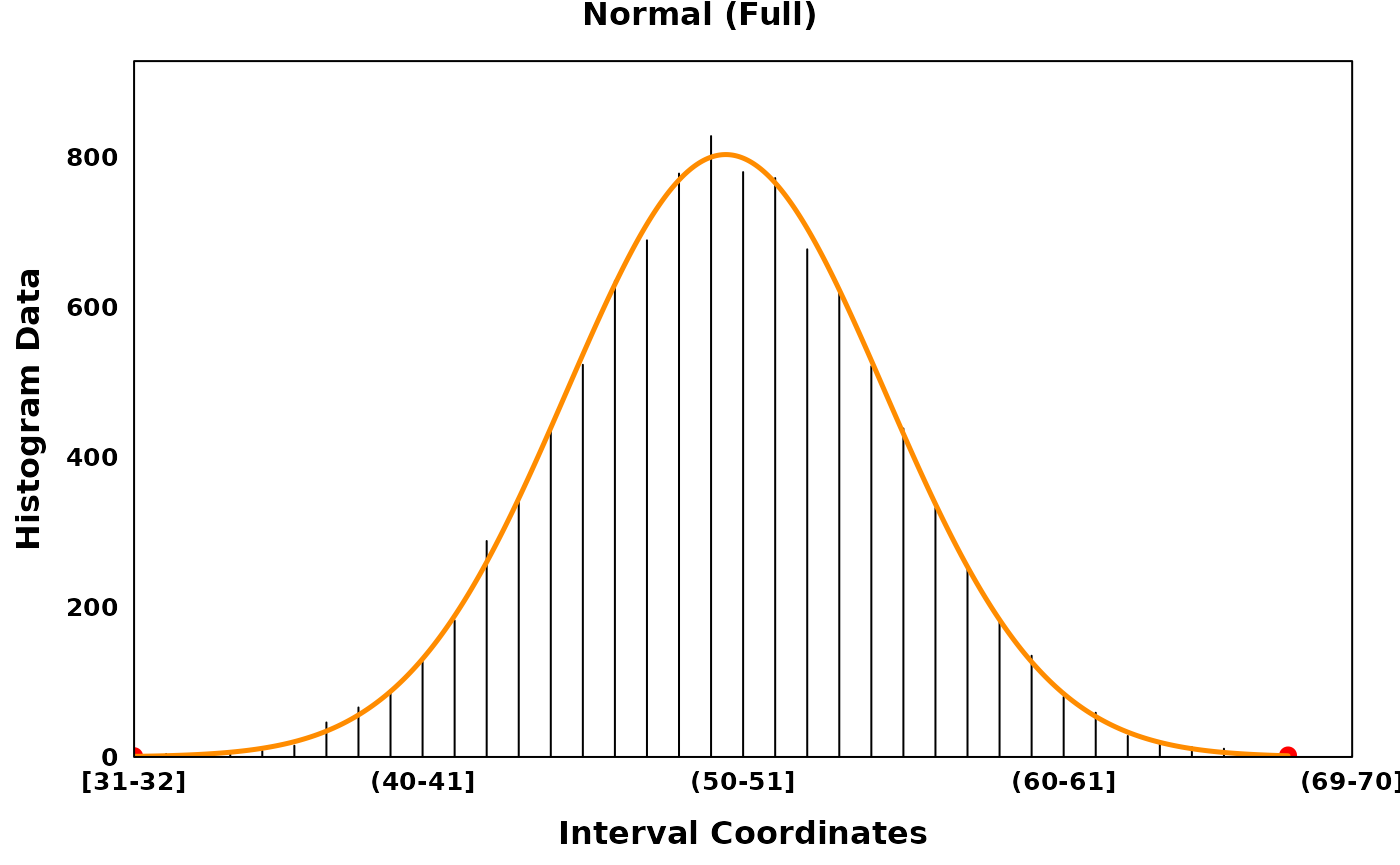

set.seed(314)
gamma_data <- rgamma(10000, shape = 2, rate = 0.4)
gamma_histogram <- observations_to_histogram(gamma_data)

# Keeping all data and fitting a full model
gamma_full <- segment_and_fit(
  histogram_obj = gamma_histogram,
  eps = 1,
  seed = 314,
  remove_low_entropy = FALSE,
  truncated_models = FALSE,
  metric = c("jaccard", "intersection", "ks", "mse", "chisq")
)

# Removing noisy data and fitting a truncated model
gamma_truncated <- segment_and_fit(
  histogram_obj = gamma_histogram,
  eps = 1,
  seed = 314,
  remove_low_entropy = TRUE,
  truncated_models = TRUE,
  metric = c("jaccard", "intersection", "ks", "mse", "chisq")
)

gamma_full_plt <- create_coverageplot(
  gamma_full,
  main = "Gamma (Full)",
  main.cex = 1, 
  xaxis.tck = 0, 
  yaxis.tck = 0, 
  xlab.cex = 1, 
  ylab.cex = 1, 
  xaxis.cex = 0.8, 
  yaxis.cex = 0.8,
  legend = NULL
)

gamma_truncated_plt <- create_coverageplot(
  gamma_truncated,
  main = "Gamma (Truncated)",
  main.cex = 1, 
  xaxis.tck = 0, 
  yaxis.tck = 0, 
  xlab.cex = 1, 
  ylab.cex = 1, 
  xaxis.cex = 0.8, 
  yaxis.cex = 0.8,
  legend = NULL
)

print(gamma_full_plt)
print(gamma_truncated_plt)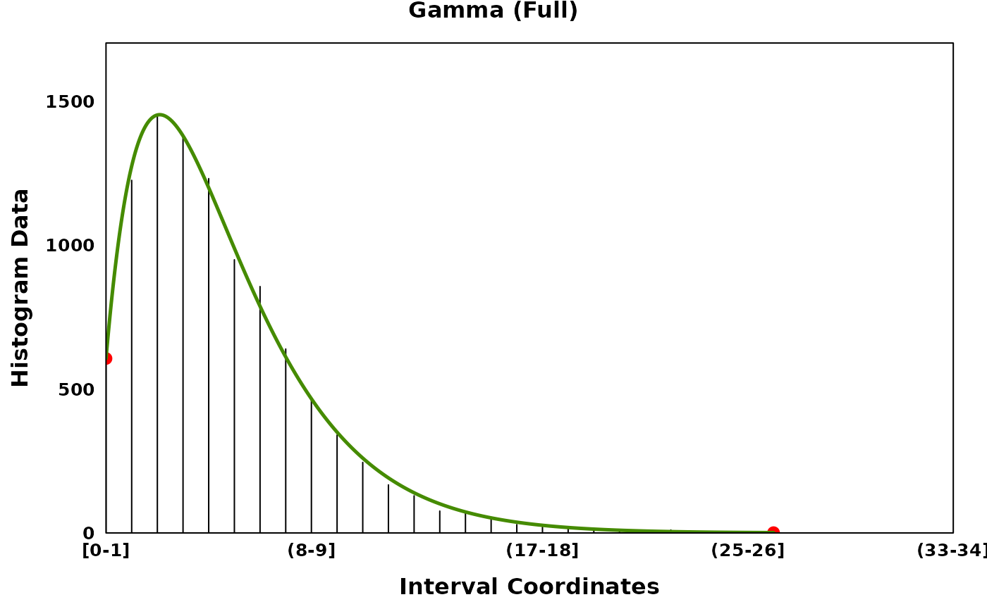

set.seed(314)
gamma_flip_data <- rgamma_flip(9000, shape = 4, rate = 0.4) + 80
gamma_flip_histogram <- observations_to_histogram(gamma_flip_data)

# Keeping all data and fitting a full model
gamma_flip_full <- segment_and_fit(
  histogram_obj = gamma_flip_histogram,
  eps = 1,
  seed = 314,
  remove_low_entropy = FALSE,
  truncated_models = FALSE,
  metric = c("jaccard", "intersection", "ks", "mse", "chisq")
)

# Removing noisy data and fitting a truncated model
gamma_flip_truncated <- segment_and_fit(
  histogram_obj = gamma_flip_histogram,
  eps = 1,
  seed = 314,
  remove_low_entropy = TRUE,
  truncated_models = TRUE,
  metric = c("jaccard", "intersection", "ks", "mse", "chisq")
)

gamma_flip_full_plt <- create_coverageplot(
  gamma_flip_full,
  main = "Gamma Flipped (Full)",
  main.cex = 1, 
  xaxis.tck = 0, 
  yaxis.tck = 0, 
  xlab.cex = 1, 
  ylab.cex = 1, 
  xaxis.cex = 0.8, 
  yaxis.cex = 0.8,
  legend = NULL
)

gamma_flip_truncated_plt <- create_coverageplot(
  gamma_flip_truncated,
  main = "Gamma Flipped (Truncated)",
  main.cex = 1, 
  xaxis.tck = 0, 
  yaxis.tck = 0, 
  xlab.cex = 1, 
  ylab.cex = 1, 
  xaxis.cex = 0.8, 
  yaxis.cex = 0.8,
  legend = NULL
)

print(gamma_flip_full_plt)
print(gamma_flip_truncated_plt)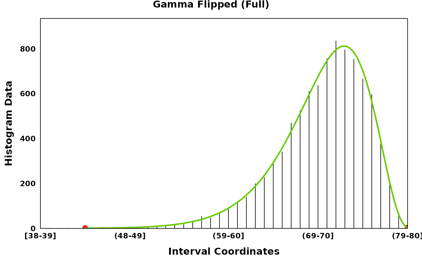

set.seed(314)
uniform_data <- runif(10000, min = 0, max = 10)
uniform_histogram <- observations_to_histogram(uniform_data)

# Fitting a uniform segment
uniform_fit <- segment_and_fit(
  histogram_obj = uniform_histogram,
  eps = 1,
  seed = 314,
  max_uniform = FALSE,
  metric = c("jaccard", "intersection", "ks", "mse", "chisq")
)

uniform_plt <- create_coverageplot(
  uniform_fit,
  main = "Uniform",
  main.cex = 1, 
  xaxis.tck = 0, 
  yaxis.tck = 0, 
  xlab.cex = 1, 
  ylab.cex = 1, 
  xaxis.cex = 0.8, 
  yaxis.cex = 0.8,
  legend = NULL
)

print(uniform_plt)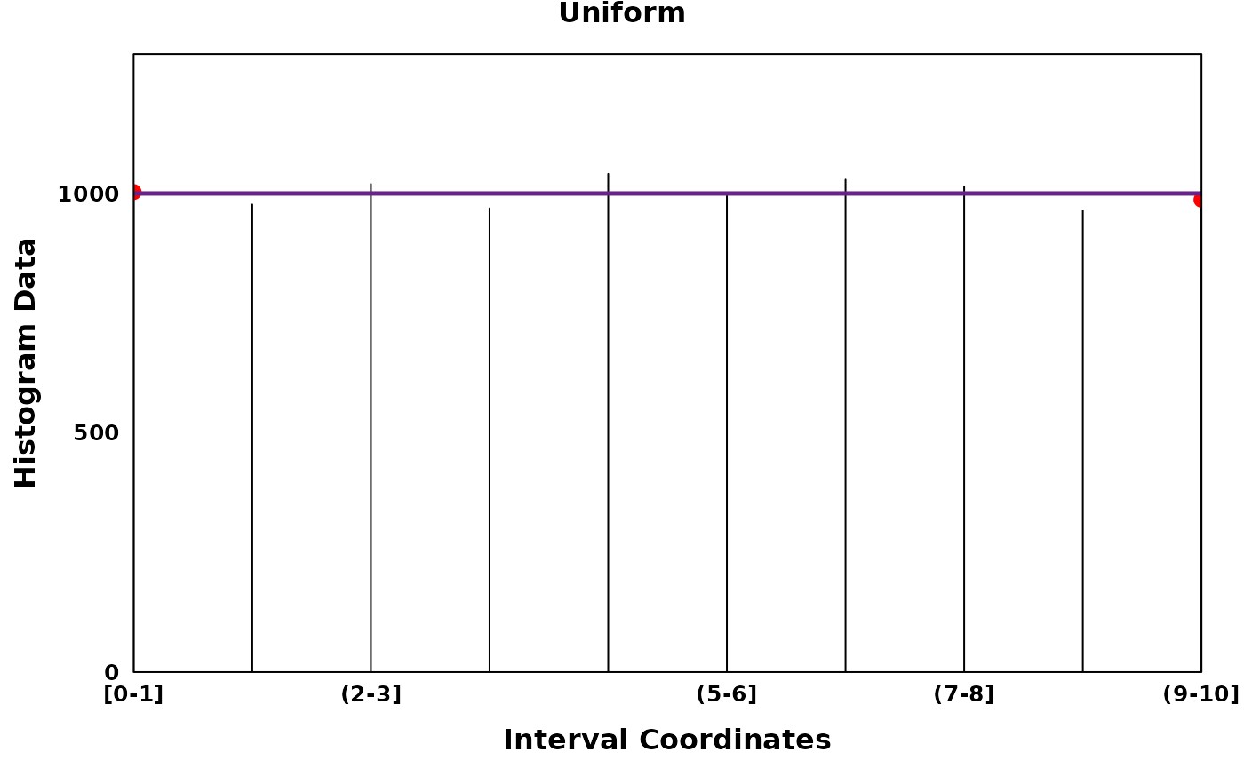

Metrics

HistogramZoo provides alternative estimators based on histogram distance for distribution parameters. Five potential metrics are available and parameters are selected to minimize the error between the density function of a statistical distribution and the observed histogram density. A full collection of histogram comparison metrics is described by (Meshgi and Ishii 2015).

Let \(h\) be our observed histogram, where \(h(i)\) is the density at bin \(i\) and \(x(i)\) be the mid-point for the bin \(i\). We define the histogram metrics, compared to a distribution \(f\) as follows:

Jaccard index is the ratio between the intersection of the fitted and observed distributions and the union of the two distributions. When comparing two histograms, intersection is the minimum and union is the maximum.

\[ D_{J}(h, f) = 1 - \frac{\sum_{i=1}^{n}\min\left(h(i), f(x(i))\right)}{\sum_{i=1}^{n}\max\left(h(i), f(x(i))\right)} \]

Intersection is the intersection between the fitted and observed distributions

\[ D_{\cap} = 1 - \frac{\sum_{i} \left(\min(h(i),f(x(i)) \right)}{\min\left(\vert h(i)\vert,\vert f(x(i)) \vert \right)} \]

Kolmogorov-Smirnov statistic is the maximum divergence between the fitted and observed distributions.

\[ D_{KS}(h, f) = \max_i \left|h(i) - f(x(i))\right| \]

Mean squared error is the mean squared difference between the fitted and observed distributions.

\[ D_{MSE}(h, f) = \frac{1}{n}\sum_{i=1}^{n}\left(h(i) - f(x(i))\right)^2 \]

\(\chi\)-squared statistic is the \(\chi\)-squared distance between the two distributions i.e.

\[ D_{\chi^2}(h, f) = \sum_{i=1}^{n}\frac{\left[ h(i) - f(x(i)) \right]^2}{h(i) + f(x(i))} \]

Maximum likelihood estimation

Maximum likelihood estimation using histogram data (ref) is provided for distribution fitting and parameter estimation. The log likelihood of a bin is given by the following formula:

\[ \log \prod_{i = 1}^{k} (F_\theta(x_i) - F_\theta(x_0))= k\log(F_\theta(x_1) - F_\theta(x_0)) \]

where \(F_\theta\) is the cumulative distribution function of the fitted distribution with parameters \(\theta\) and \(x_i\) and \(x_0\) are the start and endpoints of a bin \((x_0, x_1]\).

Finding a consensus model

The function find_consensus_model is used to determine the best fitting model for each segment and provides two methods of doing so: weighted_majority_vote (weighted majority voting) and rra (robust rank aggregation, Kolde et al. (2012)). Weighted majority voting requires the users to provide a ranking of metrics in descending order of importance and their associated weights and used the weighted sum of ranks to determine the best fitting distribution. In the event of a tie, the highest ranked metric is used to break the tie.

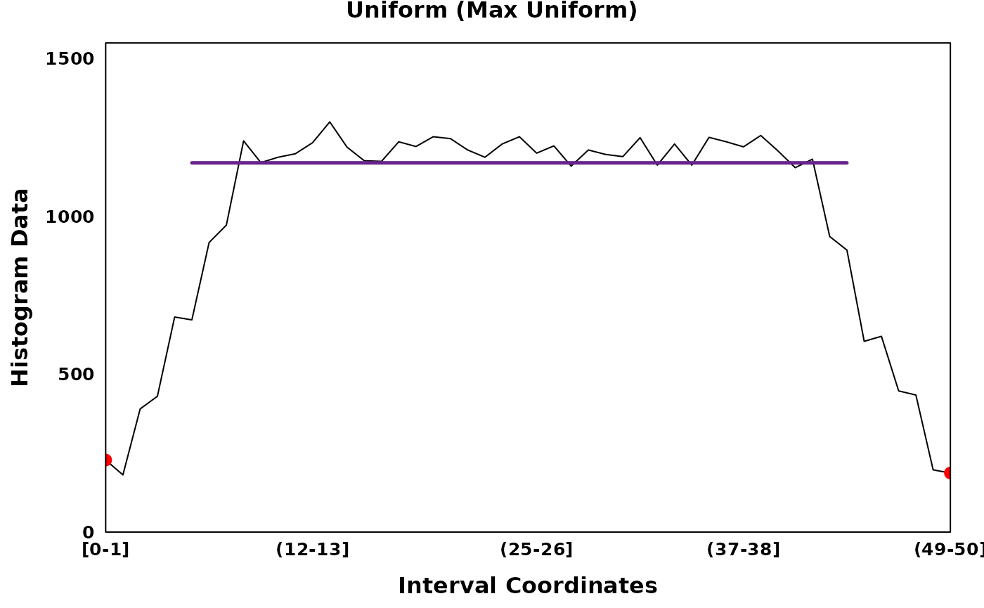
Maximizing uniform segments

The function identify_uniform_segment optimizes the identification of uniform segments by iteratively trimming the ends of the region and refitting a uniform distribution to the shortened region. This is controlled by the threshold parameter which is the proportion of the original region which must be preserved and the stepsize which indicates the stepsize taken for each search. One of the metrics must be selected to determine the best fit while the parameter max_sd_size indicates the maximum tolerable standard deviation of the goodness-of-fit from the best fitting uniform distribution where the function can select the longest uniform distribution.

set.seed(314)

# Simulating uniform data that can benefit from trimming
uniform_data <- c(
  runif(10000, min = 0, max = 50),
  runif(10000, min = 2, max = 48),
  runif(10000, min = 4, max = 46),
  runif(10000, min = 6, max = 44),
  runif(10000, min = 8, max = 42)
)
uniform_histogram <- observations_to_histogram(uniform_data)

# Fitting a uniform segment
uniform_untrimmed <- segment_and_fit(
  histogram_obj = uniform_histogram,
  eps = 1,
  seed = 314,
  max_uniform = FALSE,
  remove_low_entropy = FALSE,
  metric = c("jaccard", "intersection", "ks", "mse", "chisq")
)

uniform_trimmed <- segment_and_fit(
  histogram_obj = uniform_histogram,
  eps = 1,
  seed = 314,
  max_uniform = TRUE,
  uniform_threshold = 0.75,
  uniform_stepsize = 5,
  uniform_max_sd = 1,
  remove_low_entropy = FALSE,
  metric = c("jaccard", "intersection", "ks", "mse", "chisq")
)

uniform_untrimmed_plt <- create_coverageplot(
  uniform_untrimmed,
  main = "Uniform (Untrimmed)",
  main.cex = 1, 
  xaxis.tck = 0, 
  yaxis.tck = 0, 
  xlab.cex = 1, 
  ylab.cex = 1, 
  xaxis.cex = 0.8, 
  yaxis.cex = 0.8,
  legend = NULL
)

uniform_trimmed_plt <- create_coverageplot(
  uniform_trimmed,
  main = "Uniform (Max Uniform)",
  main.cex = 1, 
  xaxis.tck = 0, 
  yaxis.tck = 0, 
  xlab.cex = 1, 
  ylab.cex = 1, 
  xaxis.cex = 0.8, 
  yaxis.cex = 0.8,
  legend = NULL
)

print(uniform_untrimmed_plt)
print(uniform_trimmed_plt)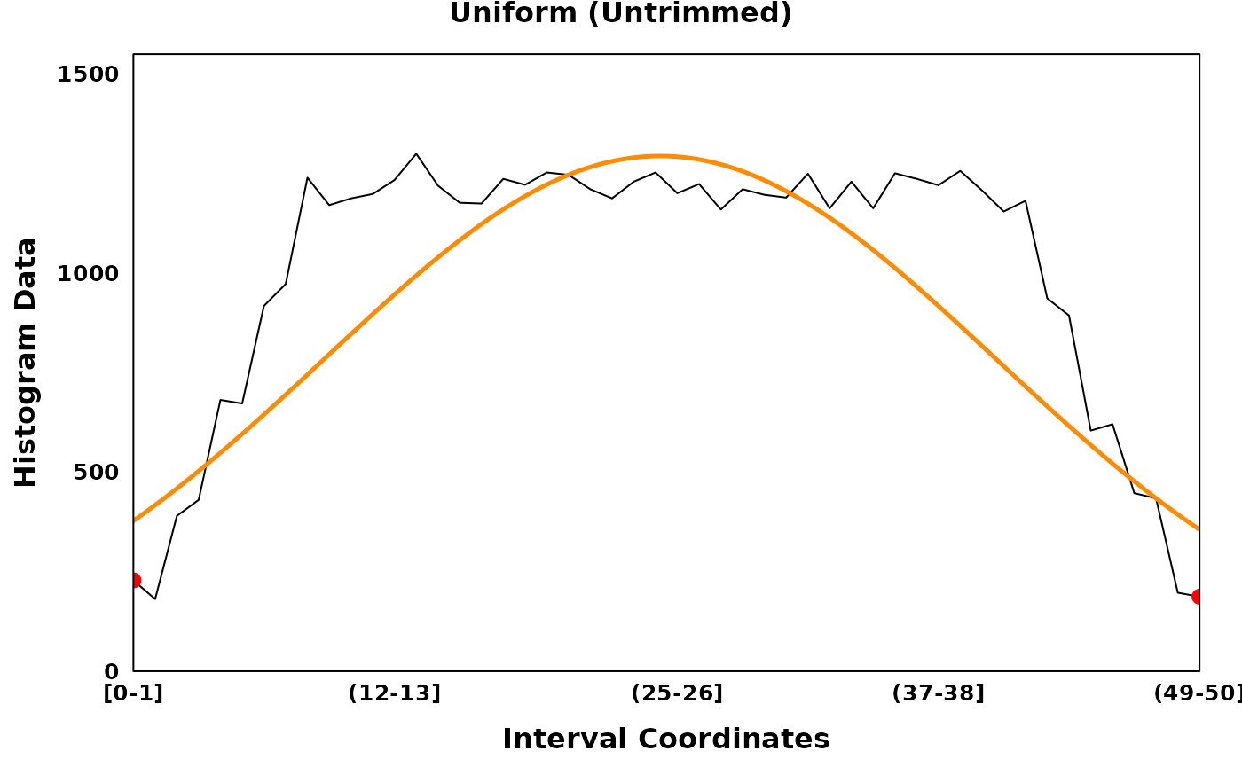

Exporting results

Summary table of results

summarize_results can be applied to a HistogramFit object to extract the indices and summary statistics of the analysis.

A data frame will be returned with the following columns.

region_id character string denoting the region_id of the Histogram
segment_id an integer id identifying the ordinal segment of the Histogram segmentation
chr an optional column denoting the chromosome of a GenomicHistogram object
start the interval start of the segment
end the interval end of the segment
strand an optional column denoting the strand of a GenomicHistogram object
interval_count the number of intervals in the segment - used for collapsing disjoint intervals
interval_sizes the width of each interval
interval_starts the start index of each interval
histogram_start The start index of the segment in the Histogram representation
histogram_end The end index of the segment in the Histogram representation
value the fitted value of the metric function
metric the metric used to fit the distribution
dist the distribution name
sample_mean the mean of the observed histogram data
sample_var the variance of the observed histogram data
sample_sd the standard deviation of the observed histogram data
sample_skew the skew of the observed histogram data
dist_param[0-9] the values of distribution parameters
dist_param_name[0-9] the matching names of distribution parameters

Plotting

Several plotting functions are available to aid with the visualization of results. Plotting functions can be combined with plotting capabilities from BoutrosLab.plotting.general (P’ng et al. 2019) based on the lattice R package (Sarkar, Sarkar, and KernSmooth 2015).

create_histogram and create_coverageplot can be used to visualize the Histogram or GenomicHistogram objects. Currently, create_coverageplot can be used to visualize HistogramFit objects, resulting from segment_and_fit analysis, with annotated segmentation points and distributions. create_histogram generates the traditional representation of histograms as consecutive blocks while create_coverageplot represents the histograms as lollipop plots or as lines. create_coverageplot was designed with large histograms, such as those derived from genomic datasets, in mind.
create_residualplot can be used to visualize the residuals between the fitted and observed distributions of a HistogramFit object
create_trackplot can be used to add complementary tracks to a histogram visualization when combined with create_layerplot
create_layerplot can be used to create a multi-panel plot with combinations of histogram, coverage, residual and track plots.

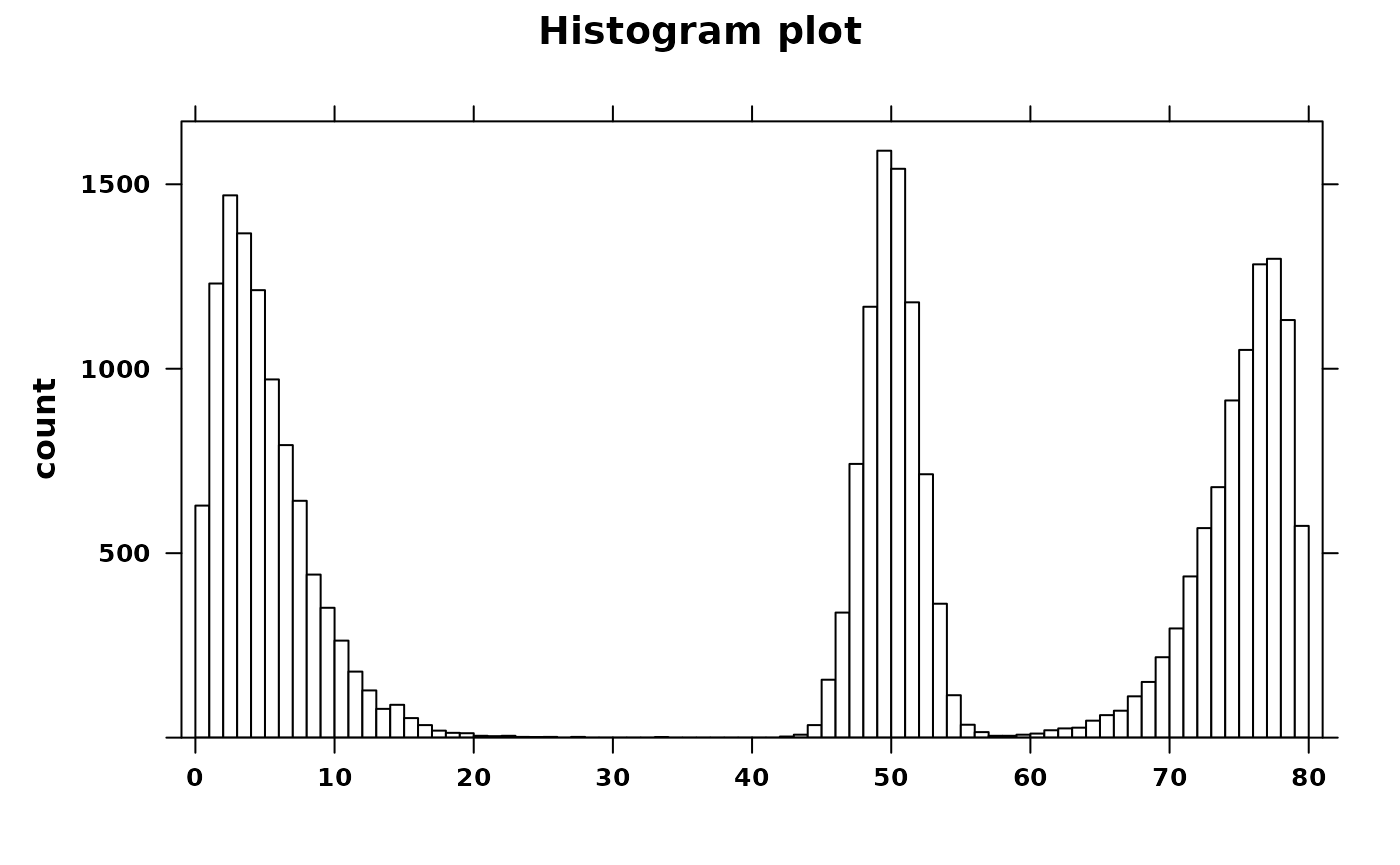
Example

A histogram is simulated from 3 statistical distributions. Two equivalent visualizations are shown below using create_coverageplot and create_histogram.

set.seed(314)
my_data <- c(
  rnorm(8000, mean = 50, sd = 2),
  rgamma(10000, shape = 2, rate = 0.4),
  rgamma_flip(9000, shape = 2, rate = 0.4) + 80
)

my_histogram <- observations_to_histogram(my_data)

# A basic coverageplot to visualize the data
create_coverageplot(
  my_histogram,
  main = "Coverage plot",
  main.cex = 1, 
  xaxis.tck = 0.5, 
  yaxis.tck = 0.5, 
  xlab.cex = 1, 
  ylab.cex = 1, 
  xaxis.cex = 0.8, 
  yaxis.cex = 0.8
)

create_histogram(
  my_histogram,
  type = "count",
  main = "Histogram plot",
  main.cex = 1, 
  xaxis.tck = 0.5, 
  yaxis.tck = 0.5, 
  xlab.cex = 1, 
  ylab.cex = 1, 
  xaxis.cex = 0.8, 
  yaxis.cex = 0.8,
  xat = seq(0, 80, 10)
)

HistogramZoo is applied to segment the histogram and fit distributions. Results are reported in a table.

# Conducting analysis
histogram_fit <- segment_and_fit(
  histogram_obj = my_histogram,
  eps = 1,
  seed = 314,
  truncated_models = TRUE,
  metric = c("jaccard", "intersection", "ks", "mse", "chisq")
)

# summarize_results to generate
res <- summarize_results(
  histogram_fit
)

The summarize_results table returns a data frame with columns describing the region_id of the original histogram and a separate for each identified segment (segment_id). The start and end columns indicate the segment indices relative to the interval_start and interval_end indices of the original histogram. The interval_count, interval_sizes and interval_starts columns aid in describing histograms with disjoint intervals following a BED file format.

knitr::kable(res[,c("region_id", "segment_id", "start", "end", "interval_count", "interval_sizes", "interval_starts")])

region_id	segment_id	start	end	interval_count	interval_sizes	interval_starts
0-80	1	0	10	1	11,	1,
0-80	2	46	54	1	9,	1,
0-80	3	71	80	1	10,	1,

The histogram_start and histogram_end columns indicate the start and end indices relative to the histogram itself (i.e. assuming that each bin is ordinal). The value refers to the GOF of the selected metric and the dist column indicates the distribution fitted.

knitr::kable(res[,c("histogram_start", "histogram_end", "value", "metric", "dist")])

histogram_start	histogram_end	value	metric	dist
1	10	0.9807606	consensus	gamma
47	54	0.9656822	consensus	norm
72	80	0.9789559	consensus	gamma_flip

The sample_mean, sample_var, sample_sd and sample_skew columns show summary statistics estimated on the observed data for each segment.

knitr::kable(res[,c("sample_mean", "sample_var", "sample_sd", "sample_skew")])

sample_mean	sample_var	sample_sd	sample_skew
4.225027	5.872675	2.423360	0.4214018
50.000982	3.111514	1.763948	0.0132582
75.984753	5.005186	2.237227	-0.3302141

The dist_param columns hold the values of the distribution parameters

knitr::kable(res[,c("dist_param1", "dist_param2", "dist_param3", "dist_param4")])

dist_param1	dist_param2	dist_param3	dist_param4
2.017559	0.3974044	0	0
50.007707	1.9119002	46	54
1.988789	0.3840282	80	0

while the dist_param_name columns hold the names of the parameters corresponding to each distribution

knitr::kable(res[,c("dist_param1_name", "dist_param2_name", "dist_param3_name", "dist_param4_name")])

dist_param1_name	dist_param2_name	dist_param3_name	dist_param4_name
shape	rate	shift	a
mean	sd	a	b
shape	rate	offset	a

A plot of the result is generated.

# Histogram Fit
coverage_plt <- create_coverageplot(
  histogram_fit,
  main = "HistogramFit",
  main.cex = 1, 
  xaxis.tck = 0, 
  yaxis.tck = 0.5, 
  xlab.label = '', 
  ylab.cex = 1, 
  xaxis.label = NULL, 
  yaxis.cex = 0.8,
  legend = NULL
)

residual_plt <- create_residualplot(
  histogram_fit,
  main = '', 
  xaxis.tck = 0, 
  yaxis.tck = 0.5, 
  xlab.label = '', 
  ylab.cex = 1, 
  ylab.label = "Residuals",
  xaxis.label = NULL, 
  yaxis.cex = 0.8
)

track_plt <- create_trackplot(
  res,
  row_id = "region_id",
  metric_id = "value",
  start_id = "histogram_start",
  end_id = "histogram_end",
  xat = generate_xlabels(histogram_fit, return_xat = T),
  xaxis.lab = generate_xlabels(histogram_fit),
  main = '', 
  xaxis.tck = 0, 
  yaxis.tck = 0, 
  xlab.cex = 1, 
  ylab.cex = 1,
  ylab.label = "GOF",
  xaxis.cex = 0.8, 
  yaxis.lab = NULL
)

covariate.legend <- list(
  legend = list(
    colours = c(
      "orange",
      "chartreuse4",
      "chartreuse3"
    ),
    labels = c(
      "Normal",
      "Gamma",
      "Gamma Flipped"
    ),
    title = expression(bold(underline('Fitted Distributions'))),
    lwd = 0.5
  ),
  legend = list(
    colours = c("red"),
    labels = c("FTC Segmentation"),
    title = expression(bold(underline('Points'))),
    lwd = 0.5
  ),
  legend = list(
    colours = c('blue', 'red'),
    labels = c(
      formatC(min(res[,"value"]), digits = 2),
      formatC(max(res[,"value"]), digits = 2)
    ),
    title = expression(bold(underline('Fit'))),
    continuous = TRUE,
    width = 3,
    tck = 1,
    tck.number = 3,
    at = c(0,100),
    angle = -90,
    just = c("center","bottom")
  )
)

side.legend <- legend.grob(
  legends = covariate.legend,
  label.cex = 0.8,
  title.cex = 0.8,
  title.just = 'left',
  title.fontface = 'bold',
  size = 2
)

summary_figure <- create_layerplot(
  plot.objects = list(coverage_plt, residual_plt, track_plt),
  plot.objects.heights = c(4,1.5,1.5),
  y.spacing = -3.5,
  ylab.axis.padding = -13,
  legend = list(
    right = list(
      x = 0.8,
      y = 1,
      fun = side.legend
    )
  ),
  right.legend.padding = 0.5,
  right.padding = 1
)

# For exporting the plot
# filename = "SummaryFigure.pdf"
# pdf(filename, width = 7, height = 7)
# print(summary_figure)
# dev.off()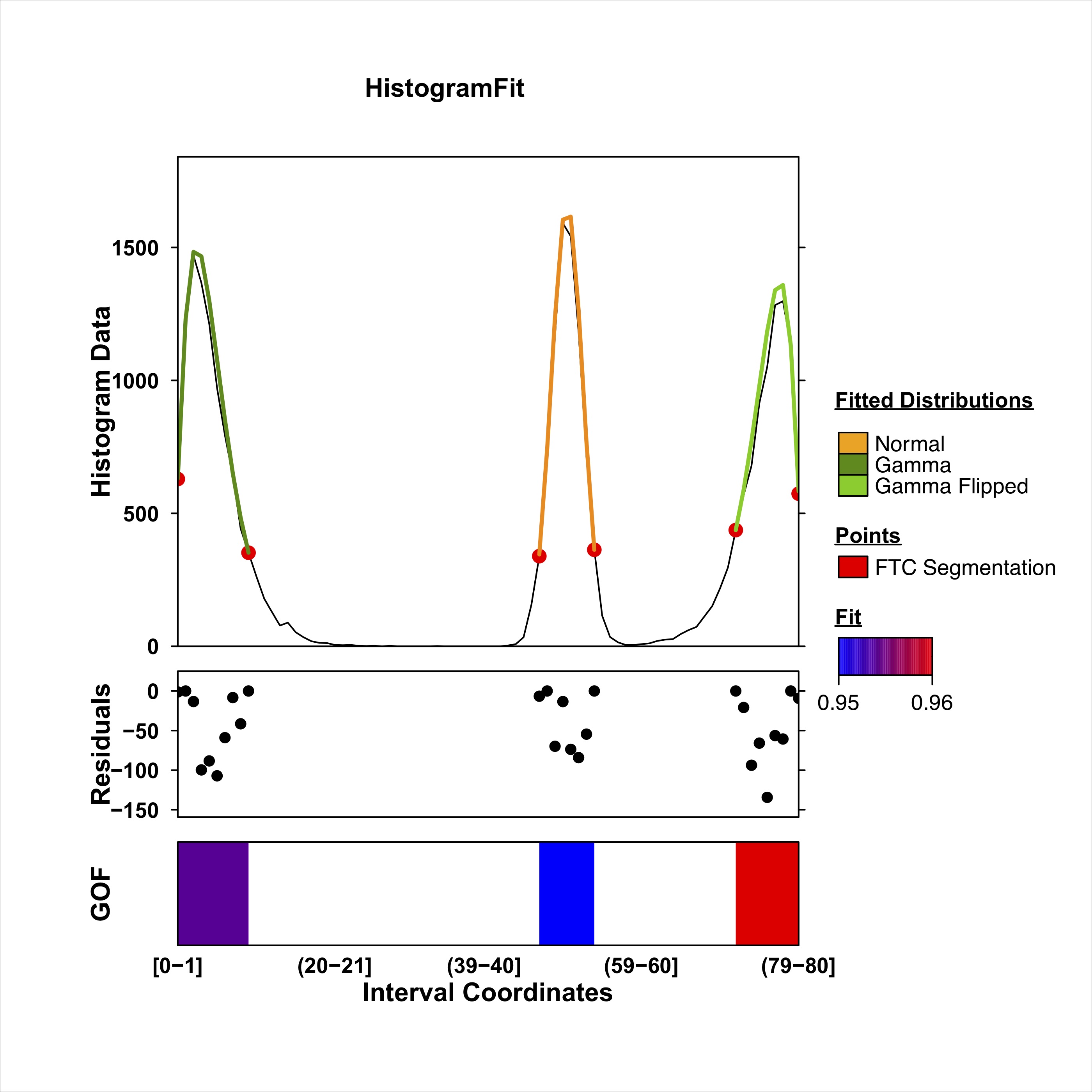

Summary Figure

References

Delon, Julie, Agnes Desolneux, Jose Luis Lisani, and Ana Belen Petro. 2005. “Color Image Segmentation Using Acceptable Histogram Segmentation.” In Iberian Conference on Pattern Recognition and Image Analysis, 239–46. Springer.

Delon, Julie, Agns Desolneux, Jos-Luis Lisani, and Ana Beln Petro. 2006. “A Nonparametric Approach for Histogram Segmentation.” IEEE Transactions on Image Processing 16 (1): 253–61.

Kolde, Raivo, Sven Laur, Priit Adler, and Jaak Vilo. 2012. “Robust Rank Aggregation for Gene List Integration and Meta-Analysis.” Bioinformatics 28 (4): 573–80.

Lisani, Jose Luis, and Ana Belén Petro. 2021. “Automatic 1D Histogram Segmentation and Application to the Computation of Color Palettes.”

Meshgi, Kourosh, and Shin Ishii. 2015. “Expanding Histogram of Colors with Gridding to Improve Tracking Accuracy.” In 2015 14th IAPR International Conference on Machine Vision Applications (MVA), 475–79. https://doi.org/10.1109/MVA.2015.7153234.

P’ng, Christine, Jeffrey Green, Lauren C Chong, Daryl Waggott, Stephenie D Prokopec, Mehrdad Shamsi, Francis Nguyen, et al. 2019. “BPG: Seamless, Automated and Interactive Visualization of Scientific Data.” BMC Bioinformatics 20 (1): 1–5.

Sarkar, Deepayan, Maintainer Deepayan Sarkar, and Suggests KernSmooth. 2015. “Package ‘Lattice’.” Version 0.20 33.

Helen Zhu & Stefan Eng