Introduction

library(PrCaMethy);

1 Background

The PrCaMethy package provides resources for predicting clinical and molecular features from prostate cancer DNA methylation data. Here is an overview of this vignette:

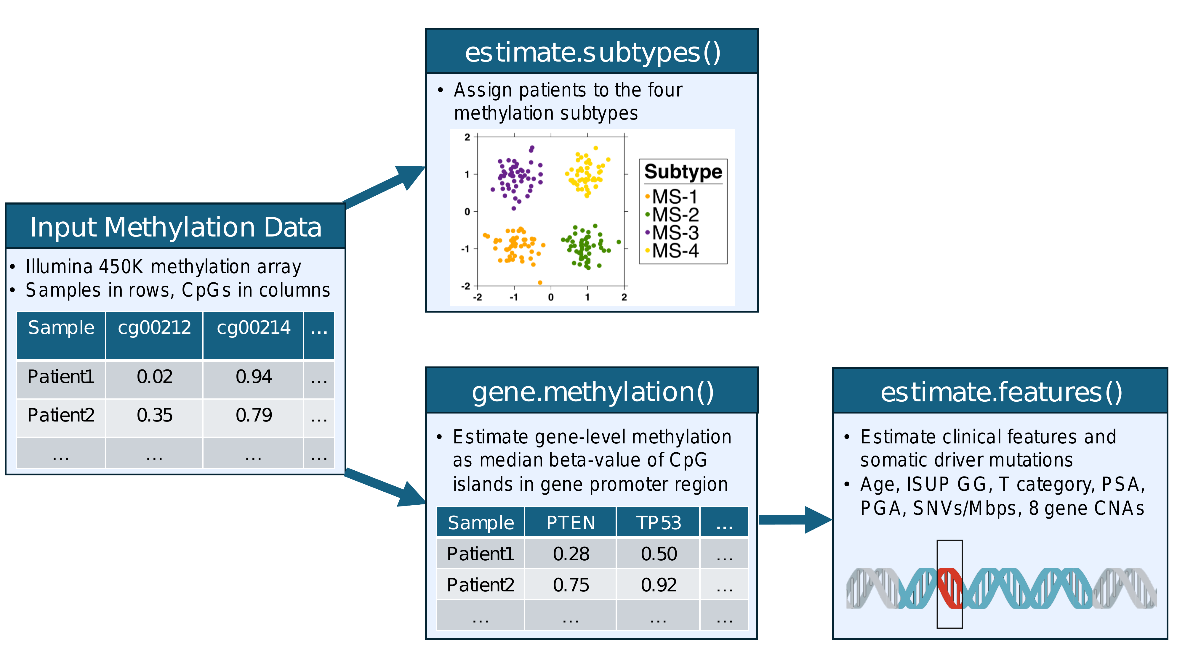
Input data explains the required format of the input data
estimate.subtypes assigns patients to one of four prostate cancer DNA methylation subtypes.
gene.methylation calculates gene-level methylation
estimate.features predicts clinical and molecular features
Quick start: putting it all together gives a concise example for how to use the functions of this package.

An overview of the 3 main R functions is shown in the diagram below:

2 Input data

Users input a data.frame containing beta-values (continuous proportions from 0 to 1) of CpG sites from the Illumina Infinium Methylation 450K BeadChip array. A list of these CpGs and their annotation data can be obtained from the IlluminaHumanMethylation450kanno.ilmn12.hg19 R package.

Ideally, the user would have all ~480k CpGs from the Illumina 450K methylation array. However, the functions in this package are written to try and estimate as many features as possible given the CpGs you have.

Here is an example dataset used throughout this tutorial:

data(example.data, package = 'PrCaMethy');
dim(example.data);

## [1]     2 93031

example.data[,1:5];

##              cg00212031 cg00214611 cg01707559 cg02839557 cg02842889
## TCGA-CH-5739  0.7147803 0.02184841 0.05281749 0.01970460  0.0284529
## TCGA-HC-7079  0.0385789 0.02315141 0.09531891 0.03250703  0.0298547

Notice the patients are in rows (rownames give patient ids) and CpGs are in columns with CpG ids as the column names.

3 `estimate.subtypes`

After making sure your methylation dataset is in the correct format (see Input data), then you can use estimate.subtypes to assign each patient to one of four prostate cancer DNA methylation subtypes (named ‘MS-1’ to ‘MS-4’). The subtypes are derived in a forthcoming manuscript.

First, let’s check whether we have the required CpGs for predicting the subtypes:

check <- validate.subtype.model.cpgs(example.data);
check$val.passed;

## [1] TRUE

check$val.passed a logical indicating whether the data passed validation
check$required.cpgs a vector of CpG ids that are required for predicting the subtypes
check$missing.cpgs a vector of CpG ids that are required but completely missing in the data
check$required.cpgs.with.high.missing a vector of CpG ids that are required and have a proportion of missing values greater than prop.missing.cutoff (default is 0.3)

Given that the validation passed, we have all required CpGs for predicting the subtypes:

subtypes <- estimate.subtypes(
    methy.data = example.data
    );
subtypes;

##              subtype
## TCGA-CH-5739    MS-3
## TCGA-HC-7079    MS-2

From our manuscript, the subtypes are interpreted as follows:

MS-1 and MS-2 had better prognosis with MS-2 being most similar to normal tissue
MS-4 had the highest risk of biochemical disease recurrence, followed by MS-3.
MS-4, followed by MS-3, had higher risk of copy number alterations, somatic driver mutations and higher global mutation density.

4 `gene.methylation`

Before we can predict other clinical and molecular features, we need to calculate gene-level methylation. Specifically, gene-level methylation is calculated as the median beta-value among CpG islands in the gene promoter region.

To calculate the gene-level methylation, you would run the following code (this may take several minutes):

example.data.gene.methy <- gene.methylation(example.data);

However, to save time, we precomputed the above dataset which you can use for the rest of the tutorial:

data(example.data.gene.methy, package = 'PrCaMethy');
dim(example.data.gene.methy);

## [1]     2 13622

example.data.gene.methy[,1:5];

##                   NIPA2       CNBP      DDX55     MRPS25      MAEL
## TCGA-CH-5739 0.02423149 0.04711574 0.02644465 0.04235761 0.9631823
## TCGA-HC-7079 0.01747738 0.04769987 0.01902647 0.03233640 0.9473169

5 `estimate.features`

Now that we have gene-level methylation data, we can predict several clinical and molecular features. The models used to predict these features were derived and validated in a forthcoming manuscript.

Currently the package supports predicting the following features:

data(all.models, package = 'PrCaMethy');
features <- names(all.models);
features <- sapply(
    X = features,
    FUN = function(x) {
      n.required.genes <- length(all.models[[x]]$xNames);
      }
    );
features <- data.frame(feature = names(features), n.required.genes = features);
rownames(features) <- NULL;
features[order(features$n.required.genes),];

##                 feature n.required.genes
## 4       psa.categorical               10
## 7       NKX3-1.cna.loss               10
## 8          MYC.cna.gain               10
## 11         RB1.cna.loss               10
## 9         PTEN.cna.loss               50
## 10      CDKN1B.cna.loss              100
## 2            ISUP.grade             1000
## 5                   pga             1000
## 6         CHD1.cna.loss             1000
## 1        age.continuous             5000
## 3            t.category             5000
## 14 log2p1.snvs.per.mbps             5000
## 12        CDH1.cna.loss            13603
## 13        TP53.cna.loss            13603

n.required.genes lists the number of required genes to predict that feature. You can see the required gene names by lapply(all.models, function(x) x$xNames).
Feature names with prefix “log2p1” means a $log_2(x + 1)$ transformation was applied.

To check whether you have the required genes to predict each feature:

check <- validate.gene.methy.data(
    gene.methy.data = example.data.gene.methy,
    models = all.models
    );

check$val.passed is a boolean vector indicating whether you have the required genes to predict all features.
check$features.you.can.predict logical vector indicating which features you can predict (i.e. you have the required genes with missing data rates < prop.missing.cutoff)
check$required.genes is a list of required genes for predicting each feature.
check$missing.genes is a list of missing genes that are required for predicting each feature.
check$required.genes.with.high.missing is a list of genes that you have but that have high missing data (i.e. proportion of missing data exceeds the cutoff to argument prop.missing.cutoff, default = 0.3)

check$val.passed;

## [1] TRUE

Given that our data passed the validation, this means we can predict all features for our dataset:

features <- estimate.features(
    gene.methy.data = example.data.gene.methy,
    models = all.models
    );

str(features$features);

## 'data.frame':    2 obs. of  14 variables:
##  $ age.continuous      : num  61.5 60.7
##  $ ISUP.grade          : Factor w/ 5 levels "ISUP1","ISUP2",..: 3 2
##  $ t.category          : Factor w/ 4 levels "T1","T2","T3",..: 3 2
##  $ psa.categorical     : Factor w/ 3 levels "psa_lt_10","psa_10_19.9",..: 1 1
##  $ pga                 : num  25.6 10.9
##  $ CHD1.cna.loss       : Factor w/ 2 levels "Yes","No": 2 2
##  $ NKX3.1.cna.loss     : Factor w/ 2 levels "Yes","No": 2 2
##  $ MYC.cna.gain        : Factor w/ 2 levels "Yes","No": 1 2
##  $ PTEN.cna.loss       : Factor w/ 2 levels "Yes","No": 2 2
##  $ CDKN1B.cna.loss     : Factor w/ 2 levels "Yes","No": 2 2
##  $ RB1.cna.loss        : Factor w/ 2 levels "Yes","No": 1 2
##  $ CDH1.cna.loss       : Factor w/ 2 levels "Yes","No": 2 2
##  $ TP53.cna.loss       : Factor w/ 2 levels "Yes","No": 2 2
##  $ log2p1.snvs.per.mbps: num  1.026 0.545

6 Quick start: putting it all together

In the previous sections, we called different validate functions to verify our data was correct. This was for educational purposes, but actually the validate functions are called automatically by other functions, thus we can simplify our code:

library(PrCaMethy);

### prepare your data
# patients are in rows (rownames give patient ids) with CpG ids as the column names.
data(example.data, package = 'PrCaMethy');
example.data[,1:5];

### predict methylation subtypes
subtypes <- estimate.subtypes(
    methy.data = example.data
    );
table(subtypes$subtype);

### calculate gene methylation data
example.data.gene.methy <- gene.methylation(example.data);
example.data.gene.methy[,1:5];

### predict clinical and molecular features
features <- estimate.features(
    gene.methy.data = example.data.gene.methy,
    models = all.models
    );
str(features$features);

Lastly, you can merge the predicted subtypes and features into a single data.frame:

results <- merge(
    x = subtypes,
    y = features$features,
    by = 'row.names',
    all = TRUE
    );
str(results);

## 'data.frame':    2 obs. of  16 variables:
##  $ Row.names           : 'AsIs' chr  "TCGA-CH-5739" "TCGA-HC-7079"
##  $ subtype             : Factor w/ 4 levels "MS-1","MS-2",..: 3 2
##  $ age.continuous      : num  61.5 60.7
##  $ ISUP.grade          : Factor w/ 5 levels "ISUP1","ISUP2",..: 3 2
##  $ t.category          : Factor w/ 4 levels "T1","T2","T3",..: 3 2
##  $ psa.categorical     : Factor w/ 3 levels "psa_lt_10","psa_10_19.9",..: 1 1
##  $ pga                 : num  25.6 10.9
##  $ CHD1.cna.loss       : Factor w/ 2 levels "Yes","No": 2 2
##  $ NKX3.1.cna.loss     : Factor w/ 2 levels "Yes","No": 2 2
##  $ MYC.cna.gain        : Factor w/ 2 levels "Yes","No": 1 2
##  $ PTEN.cna.loss       : Factor w/ 2 levels "Yes","No": 2 2
##  $ CDKN1B.cna.loss     : Factor w/ 2 levels "Yes","No": 2 2
##  $ RB1.cna.loss        : Factor w/ 2 levels "Yes","No": 1 2
##  $ CDH1.cna.loss       : Factor w/ 2 levels "Yes","No": 2 2
##  $ TP53.cna.loss       : Factor w/ 2 levels "Yes","No": 2 2
##  $ log2p1.snvs.per.mbps: num  1.026 0.545

Jaron Arbet

2025-02-26

1 Background

2 Input data

3 `estimate.subtypes`

4 `gene.methylation`

5 `estimate.features`

6 Quick start: putting it all together

Introduction

Jaron Arbet

2025-02-26

1 Background

2 Input data

3 estimate.subtypes

4 gene.methylation

5 estimate.features

6 Quick start: putting it all together

3 `estimate.subtypes`

4 `gene.methylation`

5 `estimate.features`